Basic sums and the effective conductivity of composites

Consider the effective conductivity of polydispersed fiber inclusions of conductivity \(\lambda_f\) of different sizes randomly embedded in a matrix of conductivity \(1\) (see Fig. 1).

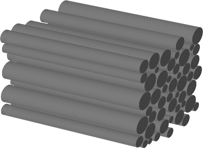
Fig. 1 Model of a polydispersed fibrous composite.

A cross–section of such composite is considered to be the periodic two–dimensional lattice \(\mathcal{Q}\), defined by complex numbers \(\omega_{1}\) and \(\omega _{2}\) on the complex plane \(\mathbb{C}\). The \((0,0)\)-cell is introduced as the parallelogram \(Q_{(0,0)}:=\{z=t_{1}\omega_{1}+t_{2}\omega_{2}:-1/2<t_{j}<1/2\;(j=1,2)\}\) (see Fig. 2).

Fig. 2 Polydispersed two–dimensional composite modelled as a two-periodic cell \(Q_{(0,0)}\).

The lattice \(\mathcal{Q}\) consists of the cells \(Q_{(m_{1},m_{2})}:=\{z\in \mathbb{C}:z-m_{1}\omega_{1}-m_{2}\omega _{2}\in Q_{(0,0)}\}\), where \(m_{1}\) and \(m_{2}\) run over integer numbers.

Inclusions are modelled by \(N\) non-overlapping disks of different radii \(r_j\) (\(j=1,2,3,\ldots,N\)). Thus, the total concentration of inclusions equals

\[\nu=\pi\sum_{j=1}^N r_j^2.\]

Let \(r=\displaystyle\max_{1 \leq j \leq N}r_j\) and introduce the constants

(1)\[\label{eq:nuConst} % \nu_j =\frac{r_j^2}{r^2}, \quad j=1,2,3,\ldots,N, \nu_j =\left(\frac{r_j}{r}\right)^2, \quad j=1,2,3,\ldots,N\]

describing polydispersity of inclusions. V.Mityushev [2] obtained the closed form representation of the effective conductivity (see also [3])

(2)\[\label{eq:eff1} \lambda=1 +2\rho \nu \sum_{q=0}^{\infty }B _{q}\nu^{q},\]

where

\[\label{eq:rho} \rho=\frac{\lambda_f-1}{\lambda_f+1}\]

is the Bergman’s contrast parameter  and the constants \(B_q\) are given by the following theorem, as linear combinations of basic sums (defined later in this section).

Theorem [1] The algorithm for generating the symbolic representations of the coefficients \(B_q\) takes the form of a recurrence relation of the first order:

(3)\[\begin{split}\label{eq:2.18} \begin{array}{lll} B_0=1&\\ B_1=\pi^{-1}\rho e_{2}, & \\ B_2=\pi^{-2}\rho^2 e_{2,2}, & \\ B_q=\pi^{-1}\beta B_{q-1}, & q=3,4,5..., \end{array}\end{split}\]

where \(\beta\) is the substitution operator modifying every basic sum in \(B_{q-1}\) according the transformation rule:

(4)\[\label{mainRule} e_{p_1,p_2,\ldots,p_n}\longmapsto\rho e_{2,p_1,p_2,\ldots,p_n}-\frac{p_2}{p_1-1}e_{p_1+1,p_2+1,p_3,\ldots,p_n}.\]

Consider a set of points \(a_k\) \((k= 1, 2,3,\ldots, N)\) in the cell \(Q_{(0,0)}\). Let \(n\) be a natural number; \(k_0, k_1\ldots, k_n\) be integers from 1 to \(N\); \(k_j\geq 2\). Let \(\mathbf{C}\) be the operator of complex conjugation. The following sums, encountered in (3)  and (4), were introduced by V.Mityushev:

(5)\[\begin{split}%\label{eq:eSum} \begin{array}{c} e^{\nu_0,\nu_1,\nu_2,\ldots,\nu_n}_{p_1,p_2,p_3,\ldots,p_n}= \displaystyle{\frac{1}{\eta^{\delta+1}} {\sum_{k_0,k_1,\ldots,k_n}}} \nu^{t_0}_{k_0}\nu^{t_1}_{k_1}\nu^{t_2}_{k_2}\cdots\nu^{t_n}_{k_n} E_{p_1}(a_{k_0}-a_{k_1})\overline{E_{p_2}(a_{k_1}-a_{k_2})}\\ \times E_{p_3}(a_{k_2}-a_{k_3})\cdots \mathbf{C}^{n+1} E_{p_n}(a_{k_{n-1}}-a_{k_n}), \end{array}\end{split}\]

where \(\eta=\sum_{j=1}^N\nu_j\) and \(\delta ={\frac{1}{2}\sum^n_{j=1}p_j}\). Functions \(E_k\) (\(k=2,3\ldots\)) are Eisenstein functions corresponding to the two-periodic cell \(Q_{(0,0)}\) (see section on Eisenstein functions), and the superscripts \(t_j\) \((j=0,1,2\ldots,n)\) are given by the recurrence relations

\[\begin{split}\label{eq:ep2nuk} \begin{array}{ll} t_0=1, \\ t_j=p_j-t_{j-1},\quad & j=1,2,3,\dots,n. \end{array}\end{split}\]

The sum (5)  is called the basic sum of the multi-order \({\mathbf p}=(p_{1},\ldots,p_{n})\). Hereafter, the superscripts for basic sum are omitted for the purpose of conciseness. In addition, following  we have \(t_n=1\). From the above definitions we see that every coefficient \(B_q\) (\(q=1,2,3, \ldots\)) forms the linear combination of basic sums. All basic sums included in the coefficient \(B_q\) are called basic sums of order \(q\).

In case of the composite modelled by \(N\) identical disks, where \(\nu_j=1\) (\(j=1,2,3,\ldots,N\)), basic sums \(e_2\) and \(e_{2,2}\) take the following forms:

\[\begin{split}\begin{array}{lll} e_{2}&= & \displaystyle{\frac{1}{N^2}} \displaystyle{\sum_{k_0=1}^{N}}\;\displaystyle{\sum_{k_1=1}^{N}}E_{2}(a_{k_0}-a_{k_1}),\\ e_{2,2}&= & \displaystyle{\frac{1}{N^3}} \displaystyle{\sum_{k_0=1}^{N}}\;\displaystyle{\sum_{k_1=1}^{N}}\;\displaystyle{\sum_{k_2=1}^{N}}E_{2}(a_{k_0}-a_{k_1})\overline{E_{2}(a_{k_1}-a_{k_2})}. \end{array}\end{split}\]

References

[1]	Nawalaniec, Algorithms for computing symbolic representations of basic e–sums and their application to composites, Journal of Symbolic Computation, Vol. 74, 328345,2016.

[2]	Berlyand, V. Mityushev, Generalized Clausius–Mossotti formula for random composite with circular fibers. J. Stat. Phys. 102 (1/2), 115–145, 2001

[3]	Gluzman, V. Mityushev, W. Nawalaniec, Computational Analysis of Structured Media. Academic Press (Elsevier), 2018