Data preparation

Note

This section is under constant development. Its content will change and improve over time.

Normalization

import matplotlib.pyplot as plt
import numpy as np

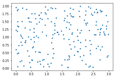
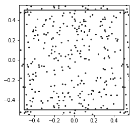
Let us generate abstract data in form of array of points (pairs of floats) bounded by a rectangle with sides of length 3 and 2 units:

W = 3
H = 2
np.random.seed(1)
data = np.random.rand(200, 2) * np.array([W, H])

plt.plot(*data.transpose(), '.')
plt.gca().set_aspect('equal')
plt.show()

In order to apply basic sums we first have to derive the complex number representation of data:

from basicsums.preparation import real_array_to_complex

data_c = real_array_to_complex(data)
data_c[:10]

array([1.25106601e+00+1.44064899j, 3.43124452e-04+0.60466515j,
       4.40267672e-01+0.18467719j, 5.58780634e-01+0.69112145j,
       1.19030242e+00+1.07763347j, 1.25758354e+00+1.370439  j,
       6.13356749e-01+1.75623487j, 8.21627796e-02+1.34093502j,
       1.25191441e+00+1.11737966j, 4.21160816e-01+0.39620298j])

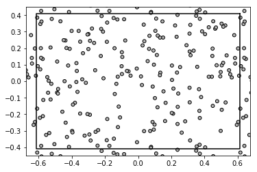
Note that structural sums operate on a subset of complex plane being a unit cell (i.e. a parallelogram with the area equal to unity). Hence, we should scale bounding box and the data. Morover, scaled bounding box should be shifted to the origin of the coordinate axes:

from basicsums.preparation import normalize_data

w1, w2, A = normalize_data(data_c, W, H)

One can check that the function returned periods of unit cell proportional to the original lengths:

w1 * w2.imag, w1/W, w2.imag/H

(1.0000000000000002, 0.4082482904638631, 0.4082482904638631)

from basicsums.show_disks import show_disks

show_disks(A, 0.01*np.ones(len(A)), w1, w2)

On the other hand, function normalize_cell_periods which returns scaled periods and the scale factor that can be used to scale the data. Note that normalize_cell_periods requires complex periods:

from basicsums.preparation import normalize_cell_periods

w1x, w2x, a = normalize_cell_periods(W, H*1j)

w1x==w1, w2x==w2, a

(True, True, 0.4082482904638631)

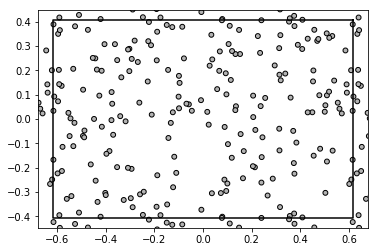
Note also that if the lengths of the sides of the bounding box are not provided, the normalize_data function figures it out based on extremal values of real and imaginary parts of data points. Hence, the automatic scale coefficient and the output period may differ from the above ones. This behaviour is usefull, when we are provided with coordinates only, without any information about the original bounding box.

w1x, w2x, Ax = normalize_data(data_c)

w1, w1x, w1x*w2x.imag

(1.2247448713915892, 1.2303484201624637, 1.0)

show_disks(Ax, 0.01*np.ones(len(Ax)), w1x, w2x)

Regularization

[TO DO]

Poisson

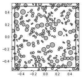
Assume that we have completelly random pattern.

from basicsums.basic_sums import Cell, BasicSums

from basicsums.show_disks import show_disks

w1, w2 = 1, 1j

qmax = 9
cell = Cell(w1, w2, qmax)
sums_indexes = [(2,)] + [(p, p) for p in range(2, qmax+1)]

N = 256
np.random.seed(10)
patterns = [np.random.rand(N, 2).dot([1, 1j]) - (0.5 + 0.5j)
            for i in range(50)]

show_disks(patterns[0], 0.005*np.ones(N), w1, w2)

res_poisson = [BasicSums(A, cell).esums(sums_indexes)
           for A in patterns]

res_poisson = np.array(res_poisson)

res_poisson.mean(axis=0)

array([-6.73534493e+00-6.85838505e-01j,  1.12429746e+06+7.21233118e-11j,
       -8.09119105e+10+8.24778547e-06j,  6.31110807e+15-2.40904496e-01j,
       -4.99712773e+20+1.17624383e+04j,  3.97136959e+25+4.73732441e+09j,
       -3.15929260e+30-1.71719493e+13j,  2.51395972e+35+1.65042148e+18j,
       -2.00059950e+40-2.67949024e+23j])

res_poisson.std(axis=0)

array([9.39936881e+01, 6.94431976e+06, 5.51104993e+11, 4.38657524e+16,
       3.49121745e+21, 2.77845506e+26, 2.21116775e+31, 1.75969592e+36,
       1.40040254e+41])

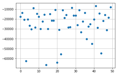
import matplotlib.pyplot as plt
k = 1
plt.plot(np.real(res_poisson[:,k]), 'o')
plt.grid(True)
plt.show()

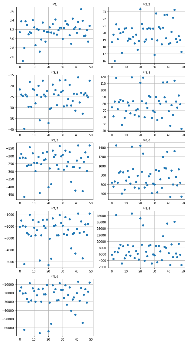
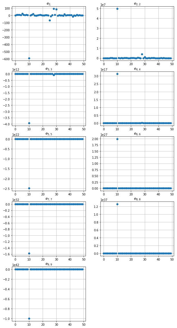
fig, ax = plt.subplots(figsize=(10, 20))
for k, tup in enumerate(sums_indexes):
    plt.subplot(5, 2, k+1)
    plt.plot(np.real(res_poisson[:,k]), 'o')
    plt.title('$e_{' + str(tup)[1:-1] + '}$')
    plt.grid(True)
plt.show()

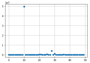
import matplotlib.pyplot as plt
k = 1
plt.plot(np.real(res_poisson[:,k]), 'o')
plt.grid(True)
plt.show()

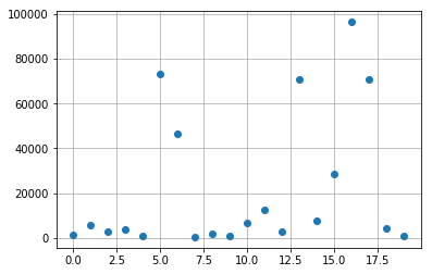
import matplotlib.pyplot as plt
k = 8
res_poisson_copy = np.copy(np.real(res_poisson[:,k]))
res_poisson_copy[10] = 0.5*(res_poisson_copy[9]+
                            res_poisson_copy[11])
plt.plot(res_d, 'o')
plt.grid(True)
plt.show()

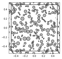
from basicsums.preparation import regularized_radii

radii = [regularized_radii(A, w1, w2) for A in patterns]

show_disks(patterns[0], radii[0], w1, w2)

show_disks(patterns[10], radii[10], w1, w2)

res_poisson_reg = [BasicSums(A, cell, r).esums(sums_indexes)
           for A, r in zip(patterns, radii)]

res_poisson_reg = np.array(res_poisson_reg)

res_poisson_reg.mean(axis=0)

array([ 3.16933109e+00+1.49275831e-02j,  1.97901593e+01-8.78395566e-17j,
       -2.50309956e+01-1.76022820e-16j,  7.87999363e+01-4.79041937e-16j,
       -2.47817891e+02+1.59840507e-16j,  7.74982714e+02-2.73951440e-15j,
       -2.41347750e+03+1.74931512e-14j,  7.65714672e+03-7.31309807e-15j,
       -2.50475199e+04+2.21614666e-13j])

res_poisson_reg.std(axis=0)

array([2.86191236e-01, 1.59002127e+00, 5.07241307e+00, 1.86463881e+01,
       8.09375185e+01, 2.82116567e+02, 1.09898397e+03, 3.92697716e+03,
       1.44629673e+04])

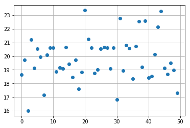
import matplotlib.pyplot as plt
k = 1
plt.plot(np.real(res_poisson_reg[:,k]), 'o')
plt.grid(True)
plt.show()

import matplotlib.pyplot as plt
k = -1
plt.plot(np.real(res_poisson_reg[:,k]), 'o')
plt.grid(True)
plt.show()

fig, ax = plt.subplots(figsize=(10, 20))
for k, tup in enumerate(sums_indexes):
    plt.subplot(5, 2, k+1)
    plt.plot(np.real(res_poisson_reg[:,k]), 'o')
    plt.title('$e_{' + str(tup)[1:-1] + '}$')
    plt.grid(True)
plt.show()