Basic sums as summary characteristics

Example 1: Visualization of dynamic changes of the system

import numpy as np

Let us import example data.

from basicsums.examples import load_example03
A_hex, r_hex, A_sqr, r_sqr = load_example03()

A_hex and A_sqr contain 128 samples of 256 equal disks of concentration 0.7 each. A_hex and r_hex represents arrays of the corresponding radii.

np.pi*sum(r_hex[0]**2), len(A_hex), len(A_hex[0])

(0.7000000000000015, 128, 256)

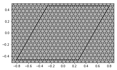
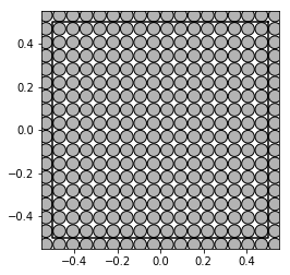
First samples of each set represent regular arrays of disks: hexagonal and square:

from basicsums.show_disks import show_disks

w1_hex = np.sqrt(2.) / (3**(1/4.))
w2_hex = w1_hex * np.exp(np.pi/3*1j)
show_disks(A_hex[0], r_hex[0], w1_hex, w2_hex)

w1_sqr = 1
w2_sqr = 1j
show_disks(A_sqr[0], r_sqr[0], w1_sqr, w2_sqr)

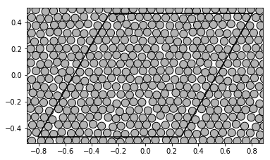
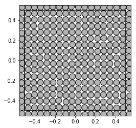
The remaining samples were created as an consequence of the random walk of the initial poisitons. Let us visualize the system after 10 steps:

t = 10
show_disks(A_hex[t], r_hex[t], w1_hex, w2_hex)
show_disks(A_sqr[t], r_sqr[t], w1_sqr, w2_sqr)

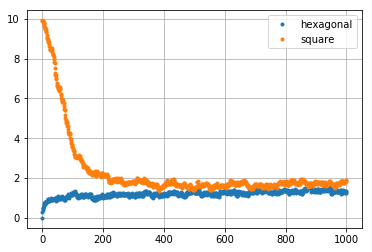
Hence, we have dynamicaly changing systems. They could model the stirr casting process [1]. Intuitively, as time of random walk aproaches infinity, both systems should converge to the same distribution (or very similar ones). Since basic sums describes geometry of such systems, the convergence should reflects in the values of certain sums. It is known that in both initial regular cases \(e_{4, 4} = S_4^2\), where \(S_4\) is a Eisenstein-Rayleigh lattice sum. Morover, \(S_4\) takes different values in both cases. Let us compute \(e_{4,4}\) for each sample:

from basicsums.basic_sums import Cell, BasicSums

qmax = 4
cell_hex = Cell(w1_hex, w2_hex, qmax)
cell_sqr = Cell(w1_sqr, w2_sqr, qmax)

You can compute the results yourself (it can take some time):

res_hex = [BasicSums(A, cell_hex, eisenstein_indexes=[4]).esum(4, 4)
           for A in A_hex]

res_sqr = [BasicSums(A, cell_sqr, eisenstein_indexes=[4]).esum(4, 4)
           for A in A_sqr]

or load them directly:

from basicsums.examples import load_example03e44
res_hex, res_sqr = load_example03e44()

Hint

One can use the tqdm package to track the progress of calculations as follows:

from tqdm import tqdm
res_hex = [BasicSums(A, cell_hex, eisenstein_indexes=[4]).esum(4, 4)
           for A in tqdm(A_hex)]

Let us create a plot of the results. One can see that the proces of changes of the random structures reflects in the real values of \(e_{4,4}\):

import matplotlib.pyplot as plt
plt.plot(np.real(res_hex), '.', np.real(res_sqr), '.')
plt.grid(True)
plt.legend(['hexagonal', 'square'])
plt.show()

Example 2: Summary characteristics of distributions of disks

Let us load another example

from basicsums.examples import load_example04
A_norm, r_norm, A_unif, r_unif = load_example04()

A_norm and A_unif contain 10 samples of 256 equal disks of concentration 0.5 each. Arrays r_norm and r_unif represents arrays of the corresponding radii.

np.pi*sum(r_norm[0]**2), len(A_norm), len(A_norm[0])

(0.5000000000000002, 10, 256)

w1, w2 = 1, 1j
show_disks(A_norm[0], r_norm[0], w1, w2)
show_disks(A_unif[0], r_unif[0], w1, w2)

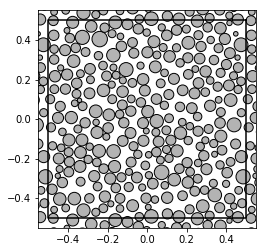
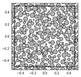
One can see, that the former samples represent disks of normally distributed radii, whereas the latter have radii drawn from the uniform distribution:

import matplotlib.pyplot as plt

fig, (ax1, ax2) = plt.subplots(2, sharex=True)
ax1.hist(r_norm.flatten(), 20)
ax2.hist(r_unif.flatten(), 20)

ax1.set_ylim([0, 350])
ax2.set_ylim([0, 350])
ax1.grid(True)
ax2.grid(True)

plt.show()

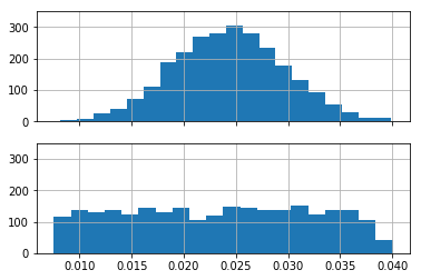
hence, we face two different distributions of disks. In order to characterize them, we need some kind of summary characteristics. Let us apply the following set of basic sums \(\{(2), (2, 2), (3, 3), (4, 4), \ldots, (9, 9)\}\) as a set of summary characteristics of distributions of disks.

qmax = 9
cell = Cell(w1, w2, qmax)
sums_indexes = [(2,)] + [(p, p) for p in range(2, qmax+1)]

Let us compute considered basic sums for each sample

res_norm = np.array([BasicSums(A, cell, r).esums(sums_indexes)
                     for A, r in zip(A_norm, r_norm)])

res_unif = np.array([BasicSums(A, cell, r).esums(sums_indexes)
                     for A, r in zip(A_unif, r_unif)])

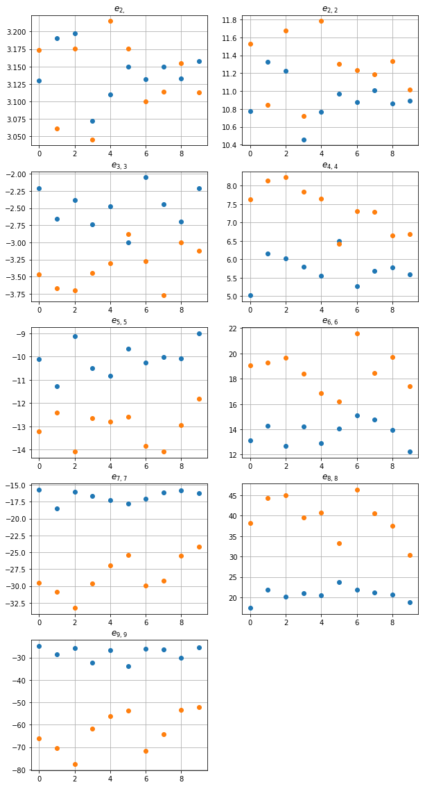
The following code creates plots of real parts of each sum:

fig, ax = plt.subplots(figsize=(10, 20))
for k, tup in enumerate(sums_indexes):
    plt.subplot(5, 2, k+1)
    plt.plot(np.real(res_norm[:,k]), 'o',
             np.real(res_unif[:,k]), 'o')
    plt.title('$e_{' + str(tup)[1:-1] + '}$')
    plt.grid(True)
plt.show()

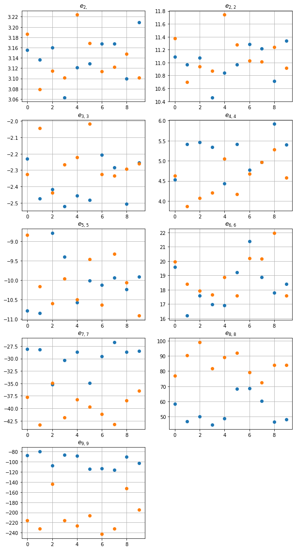
One can observe, that the larger order of the sum is, the greater difference between distributions it reveals. It is also known from the theory of composites that \(e_2 =\pi\) for macroscopically isotropic composites. Hence, one can see that both our distributions are rather isotropic.

It is known from theory of composites that \(e_2 =\pi\) for macroscopically isotropic composites. Hence, one can see that both our distributions are isotropic.

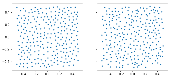
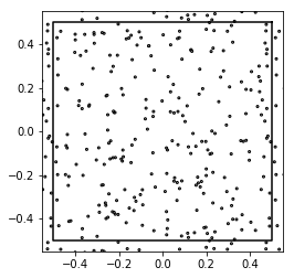
Example 3: Summary characteristics point patterns and regularization

One can consider centres of disks from the above example as point patterns, neglecting their radii.

k = 2
fig, (ax1, ax2) = plt.subplots(1, 2, sharey=True, figsize=(9, 4))
ax1.plot(np.real(A_norm[k]), np.imag(A_norm[k]), '.')
ax2.plot(np.real(A_unif[k]), np.imag(A_unif[k]), '.')
ax1.set_aspect('equal')
ax2.set_aspect('equal')
plt.show()

In order to apply basic sums as summary characteristics of point patterns, let us first present the simplest approach, i.e. to treat the points as centres of identical disks:

res_norm_points = np.array([BasicSums(A, cell).esums(sums_indexes)
                              for A in A_norm])

res_unif_points = np.array([BasicSums(A, cell).esums(sums_indexes)
                              for A in A_unif])

fig, ax = plt.subplots(figsize=(10, 20))
for k, tup in enumerate(sums_indexes):
    plt.subplot(5, 2, k+1)
    plt.plot(np.real(res_norm_points[:,k]), 'o',
             np.real(res_unif_points[:,k]), 'o')
    plt.title('$e_{' + str(tup)[1:-1] + '}$')
    plt.grid(True)
plt.show()

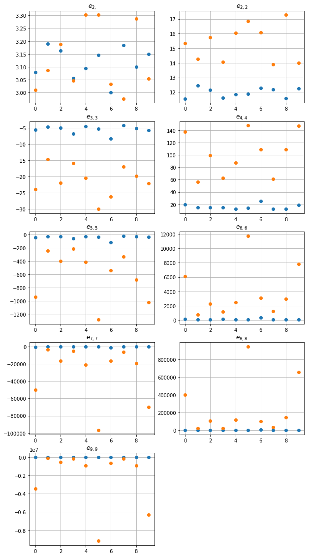
One can see, that \(e_{2,2}\) distinguishes both class of patterns very well. One can oslo observe large values of sums and deviation of the values, especiali for A_unif. This situation is common in pattern, where a very close points appear. Such a pair of points yields the difference close to zero, hence the values of \(E_n\) can be very large, since each of the functions \(E_n\) has a pole of order \(n\) at \(z=0\).

np.std(res_norm_points, axis=0)

array([9.54853920e-02, 3.06705218e-01, 1.13712103e+00, 3.96363087e+00,
       2.69872549e+01, 8.88881247e+01, 4.15380244e+02, 2.67842762e+03,
       9.78122244e+03])

np.std(res_unif_points, axis=0)

array([1.60139980e-01, 1.17750500e+00, 4.50692448e+00, 3.32374173e+01,
       3.44128094e+02, 3.35543656e+03, 2.97933172e+04, 2.98269574e+05,
       2.96228716e+06])

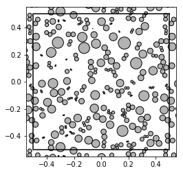
In order to obtain more stable characteristics, one can follow another schemme, where the pattern is considered as a marked one. in order to to this, we apply the regularization process, in which a set of radii (marks) is generated. For each point \(a_k\in A\) we calculate \(r_k=\frac12\min_{j\neq k}d(a_k,a_j)\) where \(d\) is a distance in the torus topology. One can consider \(r_k\) as the nearest neighbour marks.

Module basicsums.preparation contains the function regularized_radii() computing the marks:

from basicsums.preparation import regularized_radii

Let us compute regularized radii for each sample:

radii_norm = [regularized_radii(A, w1, w2) for A in A_norm]
radii_unif = [regularized_radii(A, w1, w2) for A in A_unif]

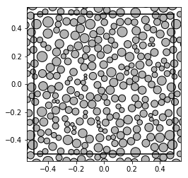
In this approach, the pattern is treated as a distribution of disks of different radii:

show_disks(A_unif[0], radii_unif[0], w1, w2)

Hence, we can calculate basic sums for each pattern:

res_norm_points_reg = np.array([BasicSums(A, cell, r).esums(sums_indexes)
                         for A, r in zip(A_norm, radii_norm)])
res_unif_points_reg = np.array([BasicSums(A, cell, r).esums(sums_indexes)
                         for A, r in zip(A_unif, radii_unif)])

This time, the deviations of the results are much smaller:

np.std(res_norm_points_reg, axis=0)

array([0.04815164, 0.22962557, 0.27581293, 0.40329808, 0.66573284,
       0.89955487, 0.87183017, 1.64641344, 2.9807516 ])

np.std(res_unif_points_reg, axis=0)

array([0.06233756, 0.32575137, 0.28875951, 0.60124032, 0.72054763,
       1.4864379 , 2.69567961, 4.80540731, 8.41615877])

fig, ax = plt.subplots(figsize=(10, 20))
for k, tup in enumerate(sums_indexes):
    plt.subplot(5, 2, k+1)
    plt.plot(np.real(res_norm_points_reg[:,k]), 'o',
             np.real(res_unif_points_reg[:,k]), 'o')
    plt.title('$e_{' + str(tup)[1:-1] + '}$')
    plt.grid(True)
plt.show()

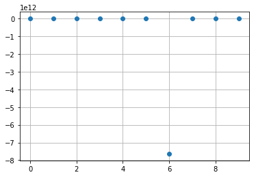
Poisson

from basicsums.show_disks import show_disks

np.random.seed(10)
patterns = [np.random.rand(256, 2).dot([1, 1j]) - (0.5 + 0.5j)
            for i in range(10)]

show_disks(patterns[0], 0.005*np.ones(256), w1, w2)

res_poisson = [BasicSums(A, cell).esums(sums_indexes)
           for A in patterns]

res_poisson = np.array(res_poisson)

res_poisson.mean(axis=0)

array([ 7.43803510e+01-3.32786887e+01j, -7.63239815e+11-7.80213066e-05j,
        7.57274786e+16+1.16441814e+00j, -7.51395614e+21-3.48134672e+03j,
        7.45563025e+26+2.41893146e+10j, -7.39775737e+31-1.44660313e+14j,
        7.34033372e+36-7.23848718e+19j, -7.28335582e+41-2.67437777e+22j])

res_poisson.std(axis=0)

array([2.37197330e+02, 2.28962306e+12, 2.27182197e+17, 2.25418678e+22,
       2.23668907e+27, 2.21932721e+32, 2.20210012e+37, 2.18500674e+42])

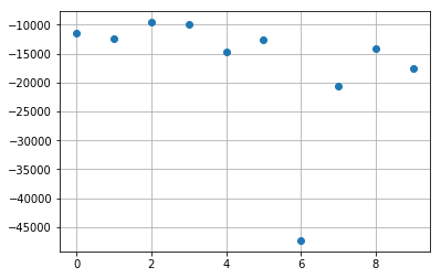
import matplotlib.pyplot as plt
k = 1
plt.plot(np.real(res_poisson[:,k]), 'o')
plt.grid(True)
plt.show()

from basicsums.preparation import regularized_radii

radii = [regularized_radii(A, w1, w2) for A in patterns]

show_disks(patterns[0], radii[0], w1, w2)

res_poisson_reg = [BasicSums(A, cell, r).esums(sums_indexes)
           for A, r in zip(patterns, radii)]

res_poisson_reg = np.array(res_poisson_reg)

res_poisson_reg.mean(axis=0)

array([ 3.09909679e+00+6.97105417e-02j, -2.24978693e+01-3.77635105e-17j,
        6.68322118e+01-4.52428521e-16j, -2.01918248e+02-3.22721685e-16j,
        6.07481859e+02+1.44567732e-14j, -1.81014006e+03+2.01664255e-14j,
        5.63754484e+03+1.53328129e-14j, -1.70439305e+04-4.07862527e-13j])

res_poisson_reg.std(axis=0)

array([3.21408956e-01, 4.24840338e+00, 1.50153967e+01, 5.80584374e+01,
       2.29771452e+02, 8.68856282e+02, 2.99968303e+03, 1.05832972e+04])

import matplotlib.pyplot as plt
k = -1
plt.plot(np.real(res_poisson_reg[:,k]), 'o')
plt.grid(True)
plt.show()

References

[1]	Kurtyka, N. Rylko, Structure analysis of the modified cast metal matrix composites by use of the RVE theory. Arch Metall. Mater 58(2), 357-360, 2013. doi: 10.2478/v10172-012-0198-x.