Computations of basic sums
For theoretical details on basic sums see Theory overview section of the online documentation and papers cited therein.
Every application of basic sums starts with a specification of the considered cell and the maximal order of sums being used (i.e. symbolic precision). Consider the square lattice and the symbolic precision \(q_\max=5\):
import numpy as np
w1, w2  = 1, 1j  # periods of the square lattice
qmax = 5         # symbolic precision
Then we create an instance of the Cell class that computes and stores the functions \(\wp\) and \(\wp'\) for a given periods \(\omega_1\), \(\omega_2\), as well as the corresponding Eisenstein functions \(E_n\) (\(n=2, 3, 4,\ldots,q_\max\)). For more details, refer to formula (5) and section Weierstrass \wp and Eisenstein functions.
from basicsums.basic_sums import Cell
cell = Cell(w1, w2, qmax)
In applications, it is common to work with sets of disks of identical or different radii. Let us investigate both cases seperately (an aproach to the analysis of points distributions is described here).
Basic sums for identical disks
Let us import a sample configuration of identical disks:
from basicsums.examples import load_example01
A, r = load_example01()
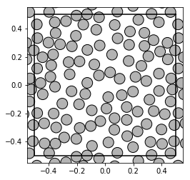
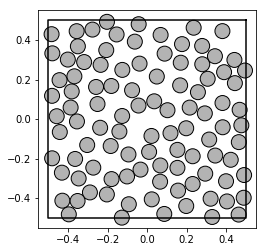
where A is a NumPy array of complex numbers specifying the disk centres and r is a NumPy array of floats corresponding to the disk radii. One can apply show_disks() function to visualize the sample:
from basicsums.show_disks import show_disks
show_disks(A, r, w1, w2)
show_disks(A, r, w1, w2, neighbs=False)
Then, for this specific configuration of disks, we create an instance of the BasicSums class, which computes all required matrices related to the functions \(E(n)\) (\(n=2, 3,4,\ldots,q_\max\)) and stores as attributes in order to reuse them in computations of basic sums (for more details on the underlying algorithms, see [1]).
from basicsums.basic_sums import BasicSums
bso = BasicSums(A, cell)
The bso object provides two main methods: esum() and
esums(). The former computes the value of a single basic sum. Let us
compute \(e_2\), \(e_{2, 5, 5}\), \(e_{3, 3, 2}\) and
\(e_{4, 4}\) seperately:
bso.esum(2), bso.esum(2, 2, 5), bso.esum(3, 3, 2), bso.esum(4, 4)
((3.15438582262448-0.09180159581592136j),
 (-0.024658672489985198+1.2585946256954157j),
 (-10.80733726705118+1.833254246831019j),
 (7.9877213504124365-2.86102294921875e-16j))
The latter, esums() method, calculates values of basic sums given by a list of tuples representing multi-indexes. The method returns a numpy array of the corresponding results:
sums = [(2,), (2, 2, 5), (3, 3, 2), (4, 4)]
bso.esums(sums)
array([  3.15438582-9.18015958e-02j,  -0.02465867+1.25859463e+00j,
       -10.80733727+1.83325425e+00j,   7.98772135-2.86102295e-16j])
We will describe the difference between the two approaches a bit later.
An instance of the BasicSums class automaticaly computes matrices of values for Eisentstein functions \(E(n)\), \(n=2, 3,4,\ldots,q_\max\) at the time of creation. On the other hand, one can optimize this process by passing the list of only those indexes of functions \(E_n(z)\) which will be used in computation:
bso = BasicSums(A, cell, eisenstein_indexes=[2, 5])
bso.esum(2, 5, 5)
(-54.5563109397971+1.4082941022526196j)
One can check which Eisenstein functions are used by a given object:
bso.eis.keys()
dict_keys([2, 5])
Disks of different radii
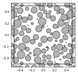
In case of disks of different radii, (i.e. polydispersed disks case), corresponding BasicSums object needs some more information about the system in the form of the normalising factors \(\nu_j, j = 1, 2, 3, \ldots, N\) (see (1)). These constants are automaticaly derived by the object based on the radii of disks. Let us import a sample with normally distributed length of radii:
from basicsums.examples import load_example02
A, r = load_example02()
show_disks(A, r, w1, w2)
Let us create the an instance of the BasicSums class:
bso = BasicSums(A, cell, r)
bso.esum(2), bso.esum(2, 3, 3)
((3.1318248855050785-0.06693636374418609j),
 (-10.346554736396879+0.9422742346896005j))
Computions of sequences of basic sums
Assume that we want to compute all basic sums from a given set, say defined by \(G'_q\) (see this section for more details). In such a case, one can use multi_indexes module implemented in the package, to get the list of required multi-indexes. Assume that we use \(G'_6\) in the following considerations:
from basicsums.multi_indexes import sums_in_Gq_prime
qmax = 5
sums = sums_in_Gq_prime(qmax)
sums
[(2,),
 (2, 2),
 (2, 2, 2),
 (3, 3),
 (2, 2, 2, 2),
 (3, 3, 2),
 (4, 4),
 (2, 2, 2, 2, 2),
 (2, 3, 3, 2),
 (3, 3, 2, 2),
 (3, 4, 3),
 (4, 4, 2),
 (5, 5)]
Let us import a random sample and create corresponding instances of Cell and BasicSums classes:
A, r = load_example01()
show_disks(A, r, w1, w2)

cell = Cell(w1, w2, qmax)
bso = BasicSums(A, cell)
One can set the dict_output parameter to True in order to force the esums() method to use a dictionary data structure (dict) instance:
sums_res = bso.esums(sums, dict_output=True)
Such an approach is very handy:
sums_res[3, 3, 2]
(-10.80733726705118+1.833254246831019j)
Moreover, it allows the transfer of the results to Pandas [2] Series or DataFrame:
import pandas as pd
pd.Series(sums_res)
2        (3.15438582262448-0.09180159581592136j)
2     (11.757827037864901+5.82076609134674e-17j)
2        (43.07907709266533-1.7681300908296955j)
3    (-3.557295937476818-7.450580596923828e-17j)
2          (173.12898896402592-6.103515625e-15j)
3        (-10.80733726705118+1.833254246831019j)
4     (7.9877213504124365-2.86102294921875e-16j)
2         (670.9285779378052-33.06492019934968j)
2           (-50.034946200507406-2.9296875e-15j)
3        (-42.96183376801067+6.393431885893068j)
3       (1.0336374840805849-1.3287290405279937j)
4        (25.69722017834029-1.0060002202097529j)
5          (-16.913965412216037+2.44140625e-16j)
dtype: complex128
Memoization and memory management
Memoization of intermediate results
What is the difference between esum() and esums() methods? Instead of computing every sum seperately via esum(), the esums() is implemented as a reccurence function that uses the momoization technique for storing vector representations (numpy arrays of \(N\) complex numbers) of intermediate sums computed during its call (for more details on algorithms and vector representations of basic sums, see [1] ). Briefly speaking, it iterates over the list of multi-indexes and computes recursively each sum, memoizing intermediate results to reuse them in computations of the remaining sums.
By default, once an intermediate vector representations of a sum is computed, it is cached in the OrderedDict data structure, so that it can be reused in the forthcoming computations Note that the cache structure is a local variable of esums(), hence all the results vanish as the function call ends.
To see this, let us derive time of computing \(G'_{16}\) containing 263167 sums:
qmax = 20
sums = sums_in_Gq_prime(qmax)
len(sums)
263167
Let us prepare the required objects:
cell = Cell(w1, w2, qmax)
bso = BasicSums(A, cell)
Now, we can compare running times of both approaches using timeit magic command:
%timeit -n 1 -r 1 np.array([bso.esum(*m) for m in sums])
1min 42s ± 0 ns per loop (mean ± std. dev. of 1 run, 1 loop each)
%timeit -n 1 -r 1 bso.esums(sums)
21.9 s ± 0 ns per loop (mean ± std. dev. of 1 run, 1 loop each)
Both the approaches give the same result.
res1 = np.array([bso.esum(*m) for m in sums])
res2 = bso.esums(sums)
np.all(np.isclose(res1, res2))
True
Intermediate vector representations are cached in the OrderedDict data structure which is local for esums() method. Hence, another run of esums() recomputes all the values. However, one can tell the esums() to store all intemediate results in the objects’s attribute:
%timeit -n 1 -r 1 bso.esums(sums, nonlocal_cache=True)
22 s ± 0 ns per loop (mean ± std. dev. of 1 run, 1 loop each)
Then,r another run computes only the sums of cached vector representations.
%timeit -n 1 -r 1 bso.esums(sums)
1.98 s ± 0 ns per loop (mean ± std. dev. of 1 run, 1 loop each)
One can check how many vector representations were stored, comparing to the number of considered basic sums:
len(sums), len(bso._cache)
(263167, 481364)
Let us clear the cache:
bso.clear_cache()
The nonlocal cache can be used in the scenario when basic sums are computed at different steps of the program. Let us first compute half of the considered sums:
half_index = len(sums)//2
%timeit -n 1 -r 1 bso.esums(sums[:half_index], nonlocal_cache=True)
len(bso._cache)
11.1 s ± 0 ns per loop (mean ± std. dev. of 1 run, 1 loop each)
240681
And the, the other half. Once the nonlocal cached was established with the nonlocal_cache parameter, it is reused and updated during the forthcomming calculations:
%timeit -n 1 -r 1 bso.esums(sums[half_index:])
len(bso._cache)
10.8 s ± 0 ns per loop (mean ± std. dev. of 1 run, 1 loop each)
481364
bso.clear_cache()
As we can see, the running times sum up to the case of calculations of all sums from sums at once.
Memory load management
Note, that the momory cache load is getting larger, as the order of \(G'_q\) increase. By default, the esums() method remembers all representations of intermediate sums. One can limit the number of cached arrays via cache_only and maxsize parameters. However, it may result in an increased running time of computations.
The cache_only parameter indicates multi-indexes of sums which should be cached.
%timeit -n 1 -r 1 bso.esums(sums, cache_only=sums, nonlocal_cache=True)
39.9 s ± 0 ns per loop (mean ± std. dev. of 1 run, 1 loop each)
The cache is much smaller now:
len(sums), len(bso._cache)
(263167, 263167)
Let us try another example:
bso.clear_cache()
%timeit -n 1 -r 1 bso.esums(sums, cache_only=sums[:5000])
1min 18s ± 0 ns per loop (mean ± std. dev. of 1 run, 1 loop each)
As we mentioned earlier, esums() uses OrderedDict for the cache. The maxsize parameter indicates that the cache will remember only maxsize most recently stored vector representations.
%timeit -n 1 -r 1 bso.esums(sums, maxsize=1000, nonlocal_cache=True)
45.2 s ± 0 ns per loop (mean ± std. dev. of 1 run, 1 loop each)
One can see, that the cache do not exceed 1000 elements:
len(sums), len(bso._cache)
(263167, 1000)
References
| [1] | (1, 2)
|
| [2] | Wes McKinney, Data Structures for Statistical Computing in Python, Proceedings of the 9th Python in Science Conference, 51-56 (2010) |